There is a way to make Bayesian predictions by simply training a single standard neural network. We call it Prior-data Fitted Networks (PFNs). As the name says, PFNs are trained on samples of prior data. That means we generate datasets from the prior and train a single neural network to make predictions one one subset of the dataset, given the rest of the dataset.
What is a Bayesian Prediction Model
We will talk about a single example of a Bayesian model, a Bayesian Neural Network (BNN).
Let’s start with the definition of what a BNN is. A BNN is a neural network where we set a (typically simple) prior on the weights. Let’s assume that our prior is that the weights are distributed like $latex p(w) = \mathcal{N}(0,\alpha \mathbb{I})$. The classical approach is to now find the posterior $latex p(w|D)$, where $D$ is a given (supervised) data set. We can find it by using $latex p(w|D) = \frac{p(D|w)p(w)}{\int p(D|w)p(w) dw}$, now we just need to know the probability of the data given a w $latex p(D|w)$, which is easy to compute for the MLP case, i.e. we feed all x in D into a neural network with weights $latex w$ and build a product of the softmax probabilities for the outputs y in D $latex \prod p(y|w,x)$.
However, to make predictions $latex p(y|x,D)$, a final integration over all weights is needed, namely $latex p(y|x,D) = \int p(w|D) p(y|w,x) dw$. $latex p(y|x,D)$ is called the posterior predictive distribution (PPD), because it is the prediction distribution that results from the posterior. In mathematics this is easy, only 2 equations. In practice, this is hard to approximate because we have two typically multi-dimensional integrals stacked on top of each other. There are methods to do it anyway (like MCMC), but they are typically very expensive per prediction, e.g. days of computation.
There are many other Bayesian prediction models. What they all have in common is that predictions are made with (an approximation of) the PPD, which is based on a prior defined in advance.
Approximation of Bayesian Predictions with PFNs
We will now explain PFNs. We will not go into the details of how they come to be approximations to the Bayesian predictions $latex p(y|x,D)$, but will save that for the next section.
PFNs are neural networks that accept a training set $latex D$ and a test input $latex x$, and they return an approximation of the the distribution of $latex p(y|x,D)$.
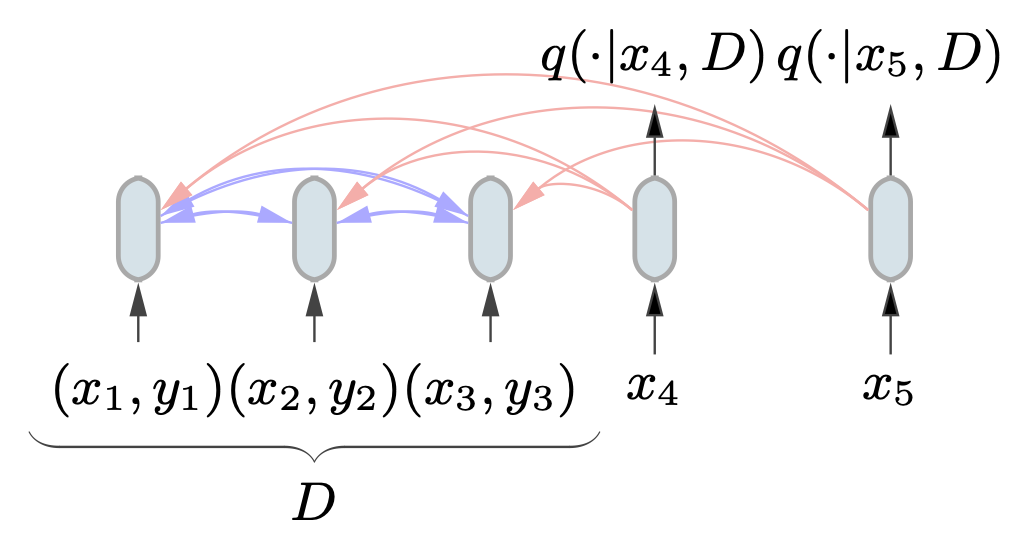
PFNs use a transformer to encode the training set $latex D$ and a set of test inputs $latex x_1,..,x_n$, as in the following figure.

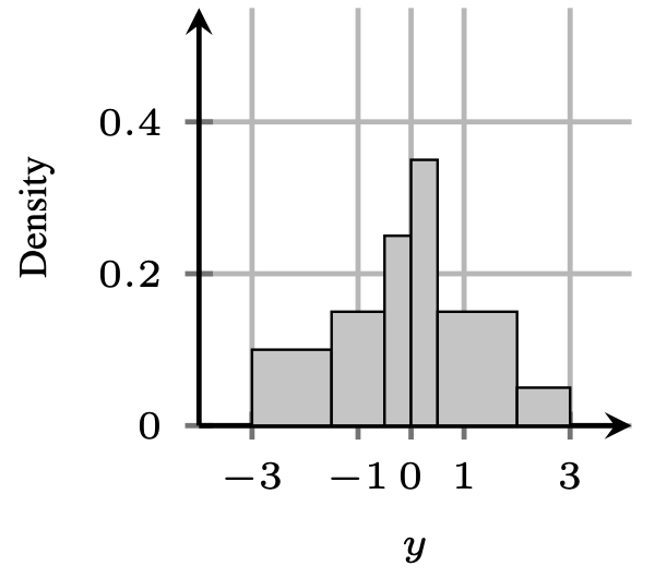
A very relevant task for PFNs is regression, as Bayesian models like Gaussian Processes are often concerned with it. We found out that it worked much better to encode regression distributions as discretized distributions, so called Riemann distributions, rather then predict a Normal distribution or similar. Our regression head, thus has a PDF over $latex y$ that looks something like below.

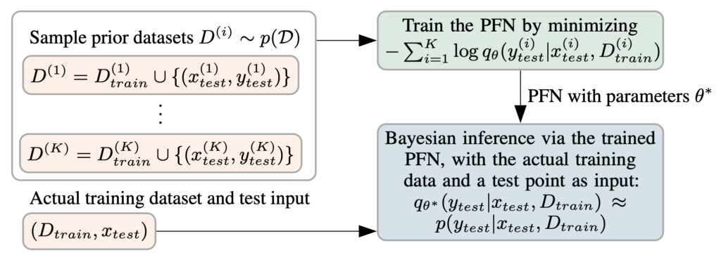
The main innovation with PFNs, though, is the way that they are trained. The weights of the PFN are actually only trained on synthetic data. That is we assume a prior, e.g. a Gaussian Process prior or a BNN prior, like above. Now we sample datasets from its prior distribution over datasets $latex p(D)$. For the BNN example that would mean, for each dataset we first sample all the weights (the latents) of the neural network from the prior. Then, we sample random inputs from a broad distribution, generally the unit cube or a standard normal, and feed them through the neural network. Finally, we feed a subset of each dataset as training set and another as test inputs for which we want to fit the outputs. Below we summarize this process in a figure.

Bayesian Interpretation of PFNs
One can actually show that PFNs trained in the way described above approximate the true posterior predictive distribution, if they are trained to the optimum and if the exact PPD is representable by the PFN architecture. In other words, the PFN training loss is exactly aligned with approximating the PPD. We show this in more detail in our initial paper.
