By Carolin Benjamins, Elena Raponi, Anja Jankovic, Carola Doerr and Marius Lindauer

TLDR: In BO: We self-adjust the exploration-exploitation trade-off online in the acquisition function, adapting to any problem landscape.

Motivation

Bayesian optimization (BO) encompasses a class of surrogate-based, sample-efficient algorithms for optimizing black-box problems with small evaluation budgets. However, BO itself has numerous design decisions regarding the initial design, the surrogate model and the acquisition function (AF). Depending on the problem at hand, a different configuration is required, directly impacting the general robustness and sample-efficiency. In this work we focus on the AF because of its direct impact on the exploration-exploitation trade-off during the search. Our method SAWEI works out-of-the-box, adapts to any problem landscape and achieves a better sample-efficiency.

Method

We propose SAWEI, Self-Adjusting Weighted Expected Improvement, to adjust the exploration-exploitation trade-off online.

For this we need three parts: (i) The adjustable acquisition function Weighted Expected Improvement (WEI) [Sobester et al., 2005], (ii) when to adjust and (iii) how to adjust.

Weighted Expected Improvement (WEI)

WEI is defined as

with $latex z(x) = (f_{min} – \hat y (x)) / \hat s (x)$, $latex f_{min}$ the lowest observed function value, $latex \hat y (x)$ and $latex \hat s (x)$ the predicted mean and standard deviation from the surrogate model and $latex \phi$ and $latex \Phi$ the PDF and CDF of a Gaussian distribution, respectively. The $latex \alpha$ coefficient weighs the exploration-exploitation terms. Depending on $latex \alpha$, we get different behaviors:

• $latex \alpha = 0.5$ recovers the standard EI [Mockus et al., 1978]
• $latex \alpha = 1$ has similar behavior as $latex PI(x) = \Phi( z(x))$ [Kushner, 1974]
• $latex \alpha = 0$ emphasizes a stronger exploration

When to Adjust?

We adjust $latex \alpha$ whenever the Upper Bound Regret (UBR) [Makarova et al., 2022] converges. The UBR estimates the true regret and is used as a stopping criterion for BO-based HPO. The gap is defined by the estimation of the worst-case function value of the best-observed point minus the estimated lowest function value across the whole search space. This means the smaller the gap becomes, the closer we are at the asymptotic function value under the current optimization settings.

When the gap falls under a certain threshold, Makarova et al. (2022) terminate the optimization. Because this threshold most likely depends on the problem at hand we use the convergence of UBR as our signal to adjust.

How to Adjust?

The remaining question is how to adjust . The convergence of the UBR is an indicator that we reach the limit of possible improvement with the current search attitude. Therefore we adjust $latex \alpha$ opposite to the current search attitude by adding or subtracting $latex \Delta\alpha$.

Experiments

We implement SAWEI in SMAC3 [Lindauer et al., 2022] and evaluate it with baselines on two well-known benchmarks for optimization: BBOB from the COCO benchmark [Hansen et al., 2021] and HPOBench [Eggensperger et al., 2021].

Key Insights

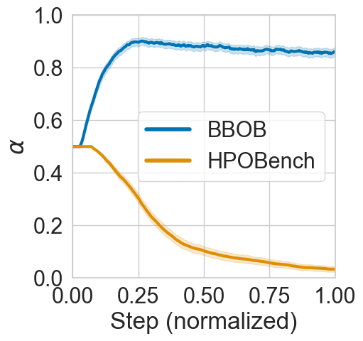
• SAWEI suitably adjust the exploration-exploitation trade-off per function and has a favorable (top 3 on BBOB and best on HPOBench) any-time performance
• On BBOB a schedule from exploration to exploitation works best
• On HPOBench a schedule from medium to maximum exploration works best, the complete opposite to BBOB

• Different baselines work well on different domains but not on both in contrast to SAWEI

Feel free to check out our paper and repository!

🌞

References

[Eggensperger et al., 2021] Eggensperger, K., Müller, P., Mallik, N., Feurer, M., Sass, R., Klein, A., Awad, N., Lindauer, M., and Hutter, F. (2021). HPOBench: A collection of reproducible multi-fidelity benchmark problems for HPO. In Proc. of NeurIPS’21 Datasets and Benchmarks Track.

[Hansen et al., 2020] Hansen, N., Auger, A., Ros, R., Mersman, O., Tušar, T., and Brockhoff, D. (2020). COCO: A platform for comparing continuous optimizers in a black-box setting. Optimization Methods and Software. 

[Kushner, 1974] Kushner, H. (1964). A new method of locating the maximum point of an arbitrary multipeak curve in the presence of noise. Journal of Fluids Engineering, pages 97–106.

[Lindauer et al., 2022] Lindauer, M., Eggensperger, K., Feurer, M., Biedenkapp, A., Deng, D., Benjamins, C., Ruhkopf, T., Sass, R., and Hutter, F. (2022). SMAC3: A versatile bayesian optimization package for Hyperparameter Optimization. JMLR, 23(54):1–9.

[Makarova et al., 2022] Makarova, A., Shen, H., Perrone, V., Klein, A., Faddoul, J., Krause, A., Seeger, M., and Archambeau, C. (2022). Automatic termination for hyperparameter optimization. AutoML Conference 2022

[Mockus et al., 1978] Mockus, J., Tiesis, V., and Zilinskas, A. (1978). The application of Bayesian methods for seeking the extremum. Towards Global Optimization, 2(117-129).

[Sobester et al., 2005] Sobester, A., Leary, S., and Keane, A. (2005). On the design of optimization strategies based on global response surface approximation models. J. Glob. Optim., 33(1):31–59.